ANIMATION OF CIRCULAR MOVEMENT - AN EXAMPLE IN PROCESSING
Processing with the java programming language, as well as the javascript variant p5js can be used to create animations of circular motion. In the following, an interactive application will be shown to display circular motion, with the ability to change the angular velocity, radius and angular acceleration. The application can be used for education and a better understanding of the kinematics of the circular movement of a material point. Also, in the following, it will be shown how a simple version of the application for circular movement can be programmed using processing.Read more about creating a circular motion simulation using p5js processing on the website:
kosi-hitac.onrender.com/en/circular-motion
Circular(rotational) movement
A circular motion can be:
- Uniform, where the angular acceleration is α=0
- Uniformly accelerated, with some non-zero angular acceleration α <>0
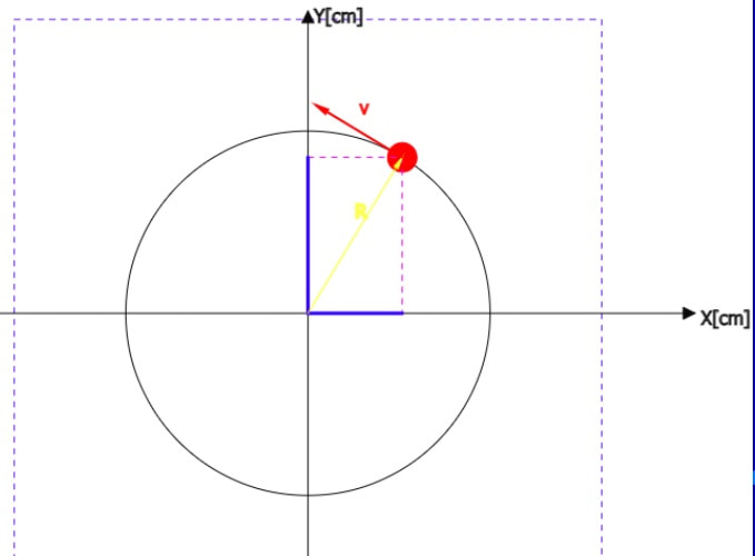
In uniform circular motion, a material point rotates along a circular path with an angular velocity that does not change over time, i.e. ω=const.
The radius vector R at every moment changes the angle coinciding with the X axis according to the law:
φ=ω * t [work]
The intensity of the linear velocity v is also constant, i.e. v=const , but the direction changes, so there is a change in the velocity vector Δv always pointing towards the center, which means there is therefore an acceleration causing this change.
It is the normal or centripetal acceleration:
aN = v2/R, or
aN = R*ω2
Unlike normal acceleration, tangential acceleration is equal to zero in uniform motion, because angular acceleration is:
α = 0
If we know the polar coordinates R and φ the position coordinates of point M, X and Y can be calculated as follows:
X=R*cos(φ)
Y=R*sin(φ)
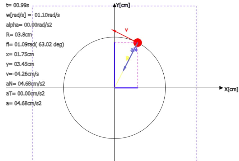
The projections of the position vector R on the coordinate axes X and Y are shown in figures 1 and 2 with blue thick lines
Figure 2 shows an example of circular motion, where ω = 1.1 rad/s and α = 0, with all displayed sizes . Velocity and normal acceleration vectors are also shown
Uniformly accelerated circular motion
In uniformly accelerated circular motion, there is an angular acceleration &alpha ><0. The angular velocity changes during time t according to the following law:
ω= ω0 + α*t
where ω0 is the angular velocity at the initial moment
Figure 2 shows an example of uniformly accelerated motion for ω = 0.5rad/s and α = 0.5 rad/s2
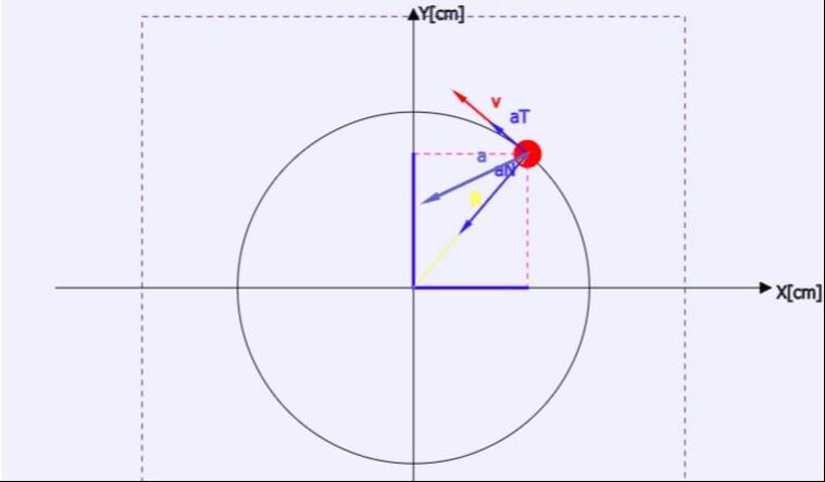
In addition to the normal acceleration, there is now a tangential acceleration aT, which always has a tangent direction, and the direction is the same as the velocity if the angular velocity increases over time, and the opposite direction if it decreases.
aT=R*α[m/s2]
Total acceleration is obtained as a vector sum of normal and tangential acceleration, as shown in Figure 3.
From the triangle formed by the vectors aN, aT and a, the intensity of the total acceleration can be determined:
a=√aN2+aT2
Circular movement - application
Below is a circular motion display application. In the blue panel, the starting values can be reduced: radius of the path R, initial angular velocity, angular acceleration using the slider. Below that is a panel with navigation buttons for start, one iteration step, pause, and reset. Also in the same panel there are "check boxes" for selecting the direction of rotation, displaying information, speed and acceleration. It is possible to slow down the animation up to 20 times, via the slow down slider, which is also located on the blue panel.Circular motion - example code in processing
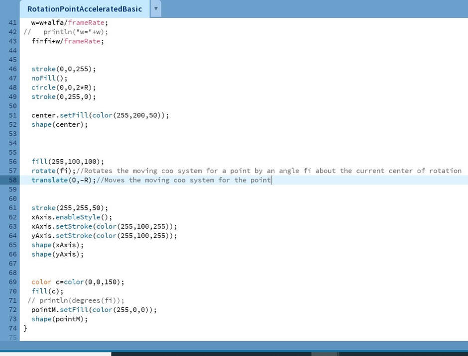
The following picture shows a simple animation of circular motion, uniformly accelerated, and then the code in processing.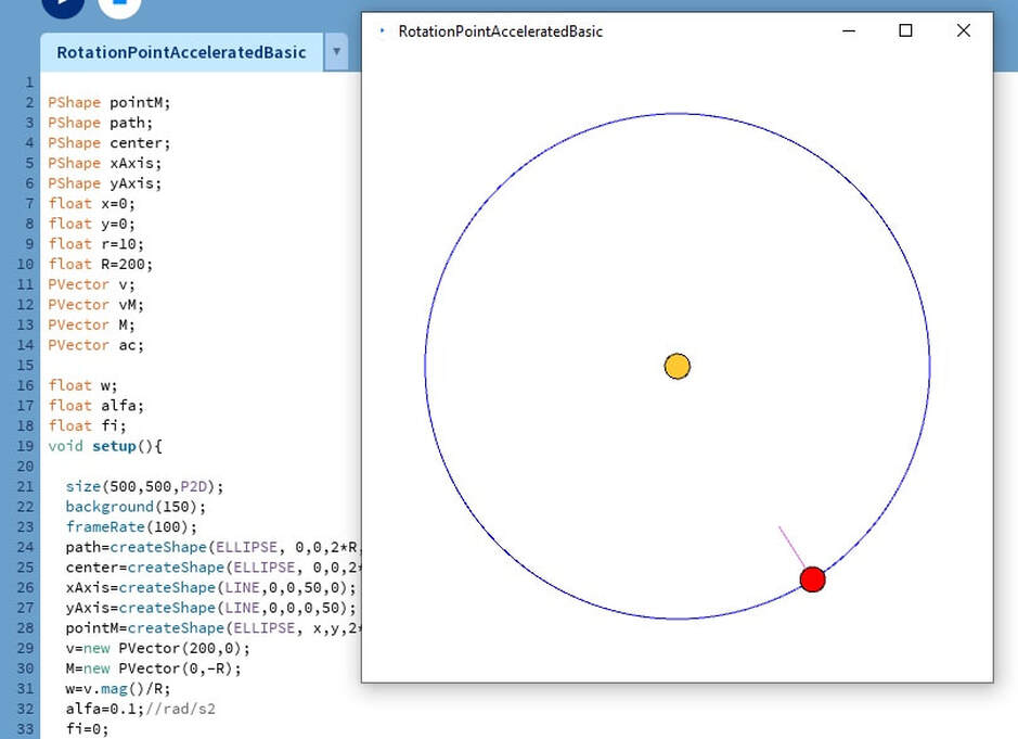
Within the setup method, the scatch size is set to 500*500, the white background, the number of iterations per second, and then the previously declared objects are created.
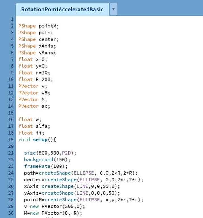
The point M is an object of class PVector, and the linear velocity v, a, w, alpha and fi are real numbers. The angular velocity w is initialized using the formula w=v.mag()/R.
The mag() function for a vector returns the intensity of the vector, as explained earlier in the article: Vectors in Processing.
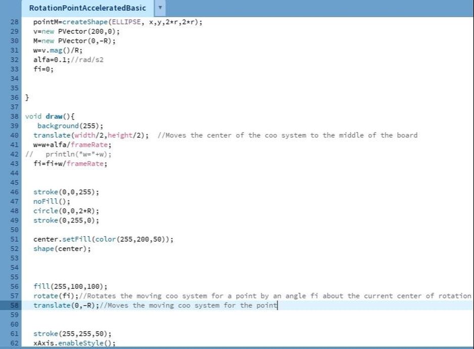
In the same method, the center, the circular path, the material point and the moving coordinate system, related to the rotating point, are then plotted.
Before drawing the small circle that rotates (point M), it is necessary to rotate the coordinate system by the angle fi, using the rotate(fi) method, and then translate it by the value -R, so that the point is then defined relative to that moving coordinate system with position coordinates (0,0).
The shape(point) method draws a point at coordinates (0,0) because these are the default coordinates, unless specified otherwise (see shape reference).