
0/1 Knapsack Problem – Dynamic Programming
The Knapsack Problem is one of the most fundamental problems in algorithm design and dynamic programming. It appears frequently in interviews and competitive programming.
What is the 0/1 Knapsack Problem?
Imagine we have a backpack with a maximum capacity of W and N items. For each item, two values are known:
- weight
w[i] - value
v[i]
Each item can be:
- taken completely
- or not taken at all
This problem often appears in optimization, combinatorics, algorithms, and programming competitions. Essentially, we are trying to find the best combination of items so that:
- the total weight does not exceed the backpack capacity W,
- the total value of the selected items is maximized
The item value (v[i]) can represent different things in practice:
- profit or price the item brings,
- utility or importance of the item,
- points, or any measurable quantitative benefit provided by the item,
- in games or simulations – strength, experience, resources, etc.
Although it sounds simple, this problem is very well-known because it is one of the classic examples of dynamic programming.
Problem Description
Given N items, where each item has:
- weight – an integer
w[i] - value – an integer
v[i]
A backpack with maximum capacity W is also given. The goal is to select a subset of items so that:
- the total weight of selected items does not exceed W,
- and the sum of their values is maximal.
Each item can be chosen at most once. Items cannot be split or taken multiple times – we either take an item completely or not at all.
Task:
Compute the maximum total value of items that can be placed into a backpack of capacity W.
Example with concrete numbersInput:
Explanation:
The optimal solution is to select items 1 and 2: total weight = 1 + 3 = 4 (≤ W), total value = 15 + 20 = 35, which is the maximum possible. Output:
The solution can be obtained using dynamic programming, either top-down (memoization) or bottom-up (tabulation). |
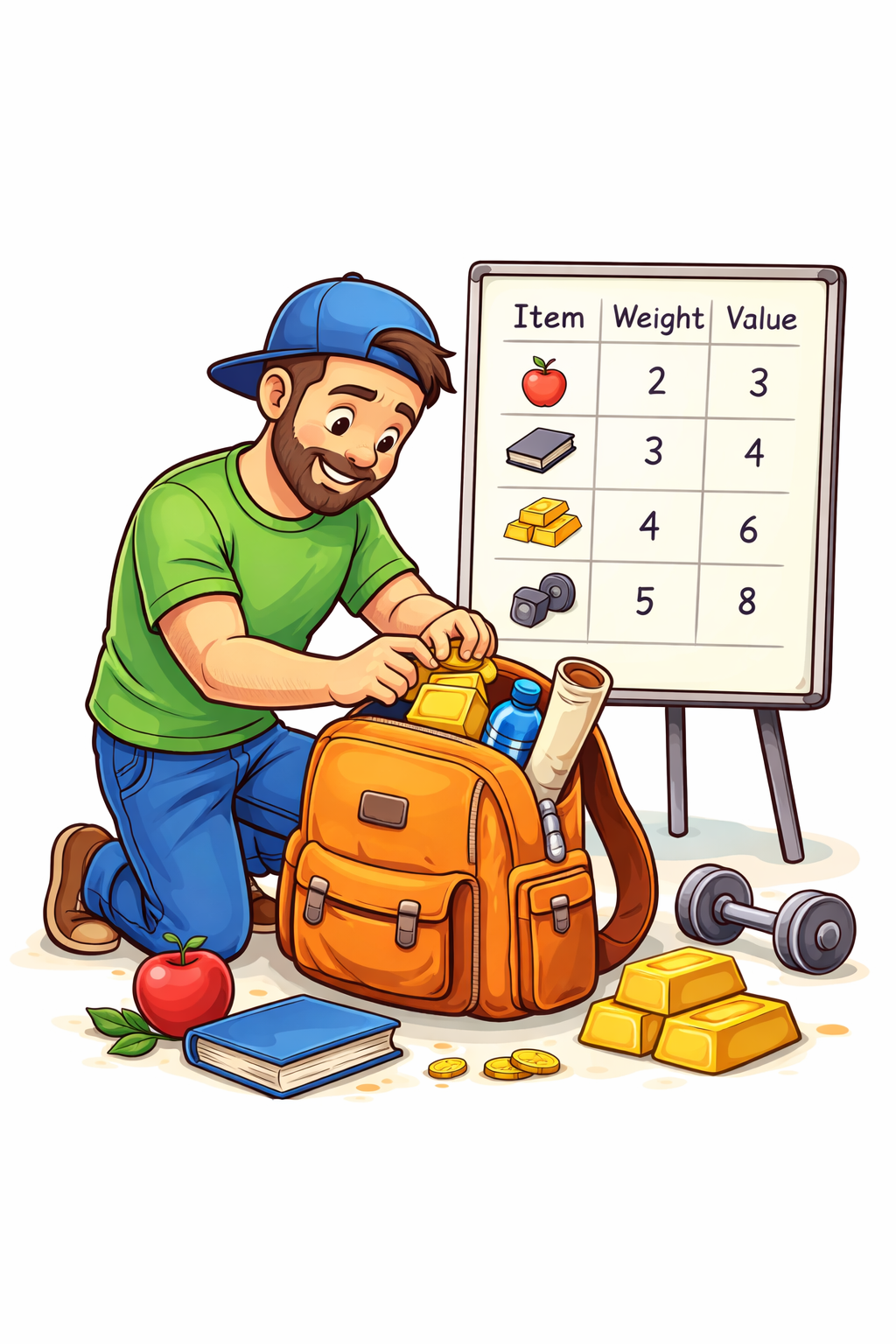
Figure 1: 0/1 knapsack problem in dynamic programming
|
Naive solution and motivation for dynamic programming
Before moving to an efficient DP solution, it is important to understand what a naive approach looks like. In the simplest version, we try all possible subsets of items (each item is either taken or not taken).
However, the number of combinations is 2^N.
For N = 30, that is already over a billion possibilities.
Therefore, the brute-force approach is far too slow and cannot be used in competitions.
This is why we introduce dynamic programming: instead of repeatedly recalculating the same subproblems, DP stores their results and uses them to solve the problem in reasonable time.
For competitions: important notes
- Pay attention to limits: always check N and W in the problem statement.
- Variable types – weights and values can often be large. Use
long longin C++. - Edge cases:
- W = 0
- N = 0
- all items heavier than W
- there is one item that exactly fits into W
- Always check if solution reconstruction is required (which items are taken).
Time complexity, limits, and when DP does not work
The standard DP solution runs in O(N · W) time.
This is much better than 2^N, but it has an important property:
the runtime depends directly on the value of W.
Therefore, we say that DP for the 0/1 Knapsack is a pseudo-polynomial algorithm – it is not polynomial in the number of input bits, but in the actual value of W.
When does the DP solution fail?
- when W is a very large number (e.g., 107, 108, or more)
- when memory cannot hold the DP table
In such cases, alternative methods are used:
- solving by values instead of weights (another DP approach)
- meet-in-the-middle (for N up to around 40)
- branch & bound or backtracking with heuristics
- approximation and FPTAS algorithms
Definition of DP state
We define:
dp[i][j] = maximum value we can achieve using
           the first i items, if the remaining knapsack capacity is j.
Base cases
dp[0][j] = 0→ With no items, the value is 0dp[i][0] = 0→ If capacity is 0, the value is 0
Transition
If the item is too heavy:
if w[i] > j:
    dp[i][j] = dp[i-1][j]
If it fits, we choose the better option:
dp[i][j] = max(
    dp[i-1][j],                 // do not take the item
    dp[i-1][j - w[i]] + v[i]    // take the item
)
C++ Implementation (with explanations)
In this program, we use dynamic programming to solve the classic 0/1 Knapsack problem. We form a DP table of size (N+1) × (W+1), where:
irepresents the first i items under consideration,jrepresents the knapsack capacity from 0 to W,dp[i][j]represents the maximum value achievable using the first i items and capacity j.
Each row of the table corresponds to including more items (1, 2, 3, ..., N).
Each column corresponds to a possible knapsack capacity (from 0 to W).
Based on this, we have two choices:
- Do not take item i — the value remains the same as dp[i-1][j]
- Take item i (if its weight ≤ j) — then consider dp[i-1][j−w[i]] + v[i]
The main goal is to find dp[N][W] — the best possible value using all items and the full knapsack capacity.
#include <iostream>
#include <vector>
using namespace std;

int main() {
    int N, W;
    cin >> N >> W;
    // N = number of items
    // W = maximum knapsack capacity

    vector<int> w(N+1), v(N+1);
    for (int i = 1; i <= N; i++)
        cin >> w[i] >> v[i];
        // w[i] = weight of the i-th item
        // v[i] = value of the i-th item

    // Create DP table of size (N+1) x (W+1)
    // dp[i][j] = best possible value using first i items and capacity j
    vector<vector<int>> dp(N+1, vector<int>(W+1, 0));

    // Fill the DP table
    for (int i = 1; i <= N; i++) {        // considering the i-th item
        for (int j = 1; j <= W; j++) {    // knapsack capacity from 1 to W

            // Option 1: Do NOT take the i-th item
            dp[i][j] = dp[i-1][j];

            // Option 2: Take the item (if it fits in the remaining capacity)
            if (w[i] ≤ j) {
                dp[i][j] = max(
                    dp[i][j],                   // do not take the item
                    dp[i-1][j - w[i]] + v[i]    // take the item
                );
            }
        }
    }

    // Final answer: best possible value with all items and full capacity
    cout << dp[N][W];
}
Example — DP Table Visualization
How is the table formed in this example?
For N = 4 items and knapsack capacity W = 7, we form a DP table with number of rows = 5 (from 0 to 4)
and number of columns = 8 (from 0 to 7).
Row i means: considering the first i items.
Column j means: maximum knapsack capacity is j.
Each cell dp[i][j] tells us: what is the maximum value achievable using items 1..i with capacity j.
Assume we have a knapsack with capacity W = 7 and 4 items:
| Item | Weight | Value |
|---|---|---|
| 1 | 1 | 1 |
| 2 | 3 | 4 |
| 3 | 4 | 5 |
| 4 | 5 | 7 |
DP table with rows corresponding to items:
| i\j | 0 | 1 | 2 | 3 | 4 | 5 | 6 | 7 |
|---|---|---|---|---|---|---|---|---|
| 0 (no items) | 0 | 0 | 0 | 0 | 0 | 0 | 0 | 0 |
| 1 (item 1: w=1, v=1) | 0 | 1 | 1 | 1 | 1 | 1 | 1 | 1 |
| 2 (item 2: w=3, v=4) | 0 | 1 | 1 | 4 | 5 | 5 | 5 | 5 |
| 3 (item 3: w=4, v=5) | 0 | 1 | 1 | 4 | 5 | 6 | 6 | 9 |
| 4 (item 4: w=5, v=7) | 0 | 1 | 1 | 4 | 5 | 7 | 8 | 9 |
Important note:
In the last cell dp[4][7], we cannot put the value 11 because that would require taking items 2 and 4:
3 + 5 = 8 > 7 — exceeds the knapsack capacity, so the combination is not allowed.
The optimal solution is to take items 2 and 3 → total value = 4 + 5 = 9.
Conclusion
The Knapsack problem is a classic contest problem because it requires understanding:
- subproblem structure
- DP state formulation
- optimal transitions
- time and memory analysis
Students who master this problem can later easily tackle:
- Unbounded Knapsack
- Subset Sum
- Coin Change
- Partition problem
Additional Materials — More Examples and Visual Explanation
To better understand the dynamic programming technique for the Knapsack problem, below is a visual representation of the DP table, an additional practice problem, and a more advanced implementation that optimizes memory to O(W).
1. Visual DP Table (Example)
Consider the following data:
- Weights: {1, 3, 4}
- Values: {15, 20, 30}
- Maximum knapsack weight: W = 4
DP table (row = number of first considered items, column = knapsack weight):
| i \ w | 0 | 1 | 2 | 3 | 4 |
|---|---|---|---|---|---|
| 0 items | 0 | 0 | 0 | 0 | 0 |
| Item 1 (1,15) | 0 | 15 | 15 | 15 | 15 |
| Item 2 (3,20) | 0 | 15 | 15 | 20 | 35 |
| Item 3 (4,30) | 0 | 15 | 15 | 20 | 35 |
The optimal solution is 35, achieved by combining items with weights 1 and 3.
Reconstructing Selected Items
After filling the DP table and calculating the maximum knapsack value,
the next important step is to reconstruct which items were actually selected.
To do this, we move backward through the DP matrix dp[i][w].
- Start from the last item:
i = nand the maximum weightw = W. - If
dp[i][w] != dp[i-1][w], then itemiwas taken. - Then decrease the weight:
w -= weight[i]. - Continue with item
i-1.
Here is a typical C++ code for reconstruction:
vector<int> reconstructItems(const vector<int>& weights,
                             const vector<int>& values,
                             const vector<vector<int>>& dp,
                             int W)
{
    int n = weights.size();
    int w = W;
    vector<int> chosen;

    for (int i = n; i > 0; i--) {
        // If the value differs, item i-1 is included
        if (dp[i][w] != dp[i-1][w]) {
            chosen.push_back(i);      // store the item index (1-based)
            w -= weights[i-1];        // decrease the remaining weight
        }
    }

    reverse(chosen.begin(), chosen.end());
    return chosen;
}
This way, we obtain the exact set of items that form the optimal knapsack solution. This step is very important because the DP table only gives the maximum value, while this procedure allows us to identify the actual items in the knapsack.
Memory Optimization — 1D DP Table
The standard solution for the knapsack problem uses a DP table of size N × W,
which can occupy a large amount of memory.
If the maximum capacity of the knapsack is large (e.g. W = 100,000), memory becomes an issue.
The good news is that the 0/1 knapsack can be optimized to use only a single dp[] array of length W+1. This reduces memory usage from O(N·W) to just O(W).
How does it work?
The key idea is that when processing item i, the DP state depends only on the previous row (i-1). Instead of storing all rows, we use a single array and update it backwards:
// dp[j] = maximum value for capacity j
vector<int> dp(W+1, 0);

for (int i = 1; i <= N; i++) {
    // important: iterate BACKWARDS to avoid overwriting needed values
    for (int j = W; j >= w[i]; j--) {
        dp[j] = max(dp[j], dp[j - w[i]] + v[i]);
    }
}
Why must we iterate backwards?
If we iterated forwards (from 0 → W), the newly updated dp[j] value would be used immediately for the next transition within the same iteration, which would incorrectly simulate the unbounded knapsack (item used multiple times).
Therefore, for the 0/1 knapsack: always iterate j from W down to w[i].
When is the 1D optimization NOT applicable?
- when you need to reconstruct the chosen subset → you must store the full 2D table (or use a separate parent array)
- when W is not too large and the 2D DP fits into memory anyway
- when solving a knapsack variant where transitions require access to DP in a different direction
Bonus Chapter — Knapsack Problem Variants
There are many versions of the knapsack problem, each with a different DP approach. These are the most important ones:
1) Unbounded Knapsack (each item can be used unlimited times)
Similar to the basic version, but transitions are calculated so that an item may be chosen more than once. The code differs in one key detail: dp is updated forwards (j from w[i] to W).
// j moves forward → the item can be used multiple times
for (int j = w[i]; j <= W; j++) {
    dp[j] = max(dp[j], dp[j - w[i]] + v[i]);
}
2) Multiple (Bounded) Knapsack — each item has a limited quantity
Each item can be used k times (e.g. you have 5 identical bottles). The solution typically uses:
- binary splitting technique (converting counts into 1,2,4,... bundles)
- or 3D DP if the counts are small
This variant lies between the 0/1 and unbounded versions.
3) Multidimensional Knapsack
Similar to the standard knapsack, but instead of one constraint (weight) there are two or more restrictions (e.g. weight and volume).
The DP is no longer 2D, but for example 3D:
// example: DP[i][w][vol]
dp[i][w][vol] = maximum value
This variant is much more demanding and is used in real-world systems (e.g. packaging, logistics, space optimization).
This chapter provides a broader view of the knapsack problem and its applications. For serious competitive programming, understanding all variants is essential.
For Competitive Programming — Key Things to Watch Out For
In competitive knapsack (Knapsack) problems, mistakes most often do not come from the DP formula itself, but from incorrect assumptions about limits and data types. Here is a short list of things you should always check before submitting a solution.
1) Limits of N and W
N— number of items (can be 1000, 5000 or more)W— maximum knapsack capacity
Before choosing the method, check the scale of the values:
- If W ≤ 2000 → standard 2D DP works without issues.
- If W ≤ 200,000 → might work with 1D optimization (if reconstruction is not required).
- If W ≥ 107 → DP becomes practically unusable (memory = problem).
2) Data Types
- Values can be large → use
long long. - The total value may exceed a 32-bit int if N is large.
- The DP table may require enormous memory → check if it fits:
dp[N+1][W+1]   →   number of elements = (N+1)*(W+1)
  • each int = 4 bytes
  • 1e8 elements → 400 MB → too much!
3) Edge Cases
N = 0orW = 0- items with weight 0 (sometimes intentionally included!)
- value = 0 (affects DP structure)
- all items heavier than W → result = 0
In many competitive problems, these inputs are exactly what cause WA (Wrong Answer) even when the main code is correct.
Algorithm Complexity and Constraints
Pseudo-Polynomial Complexity
The time complexity of the classic knapsack is:
O(N · W)
This is called pseudo-polynomial because it does not depend on the number of digits of W, but on its numeric value. If W grows by a factor of 10, the time also grows ×10.
When does DP perform poorly?
- when W is extremely large (e.g. 107 to 109)
- when the sum of weights is huge
- when memory is limited (e.g. 256MB limit in online contests)
In these situations the DP approach becomes infeasible because:
- the dp array cannot fit into memory
- execution time becomes too slow
What to use instead of DP?
If W is extremely large, competitors often switch to:
- meet-in-the-middle (for N ≤ 40)
- branch & bound techniques
- heuristics / greedy (if the problem allows it)
- bitset DP (for Subset Sum variants)
- DP over total value (when values are small, weights large)
DP Over Value (important trick!)
If the values are small (up to e.g. 103), and the weights are huge:
// dp[v] = minimum weight needed to achieve value v
This transforms the complexity from O(NW) to O(N · sum_of_values).
These observations are extremely useful for preparing for competitions such as OI, IOI, CEOI, and others. Understanding the constraints allows you to quickly identify which version of the algorithm to apply.
Hidden Mini Quiz — 0/1 Knapsack Problem
Click to test your knowledge of knapsack basics and DP solutions!
Open Quiz
Mini Quiz: Do You Understand the 0/1 Knapsack Problem?
1. What is the correct DP relation for the 0/1 Knapsack problem?
2. If W = 0 or N = 0, what will dp[N][W] be?
3. What is the main idea behind reconstructing the chosen items?
4. When is the standard DP solution pseudo-polynomial?
5. What is good practice when both W and N are large?
Practice Tasks (with instructions, without solutions)
Task 1:
A group of items is given, each with a weight and a value. Each item can be taken at most once. Determine the maximum total value that can be packed into a knapsack of capacity W = 25.
- Weights: {4, 7, 9, 12, 13}
- Values: {10, 13, 18, 22, 23}
Instruction (short):
Create a DP table of size (n+1) × (W+1) and fill it using the standard transition:
dp[i][w] = max(dp[i-1][w], dp[i-1][w - weight[i]] + value[i])
Pay special attention to the case when weight[i] > w —
then the value is simply copied from the previous row.
Before checking the solution, try on your own:
- to estimate which item combinations might fit into the knapsack
- to roughly predict the maximum possible value
2. Knapsack optimized to O(W) memory
Problem statement
The classic 0/1 Knapsack problem is given. For a knapsack capacity W and a list of items (each with weight w[i] and value v[i]), compute the maximum total value that can fit in the knapsack.
Your task is to write an optimized solution that uses only O(W) memory (a one-dimensional DP array).
Most important rule: iterate the weights backwards.
Before checking the solution, try to answer:
- Why must the weight loop go backwards?
- What would happen if we looped forwards?
3. Reconstructing the Selected Items (0/1 Knapsack)
Problem statement
After filling the dynamic programming table for the classical 0/1 Knapsack problem and computing the maximum achievable value, it is often necessary to know which exact items form that optimal solution.
You are given an already filled DP table dp[i][w], where
dp[i][w] represents the maximum value obtainable
using the first i items and knapsack capacity w.
Your task is to implement an algorithm for reconstructing the chosen items — i.e. determining which items are included in the optimal solution.
Reconstruction is performed backwards, starting from the state
i = n and w = W, by analyzing changes in the DP table.
You should write C++ code that returns the indices of the selected items (1-based) that form the optimal knapsack content.
Example inputs and expected outputs
Example 1
Input:
weights = {1, 3, 4}
values  = {15, 20, 30}
W = 7

Filled DP table (dp):
i\w | 0  1  2  3  4  5  6  7
--------------------------------
0   | 0  0  0  0  0  0  0  0
1   | 0 15 15 15 15 15 15 15
2   | 0 15 15 20 35 35 35 35
3   | 0 15 15 20 35 45 45 50

Expected output:
Selected items: 1 3
Explanation:
Item 1 (weight 1, value 15) and item 3 (weight 4, value 30)
together give the maximum value of 45 with capacity 7.
Example 2
Input:
weights = {2, 5, 3, 4}
values  = {6, 10, 7, 12}
W = 7

Expected output:
Selected items: 1 4
Example 3
Input:
weights = {4, 2, 3}
values  = {8, 5, 6}
W = 5

Expected output:
Selected items: 2 3
Before looking at the solution, think about:
- Why does comparing with
dp[i-1][w]work? - What does it mean if the values are equal?
- Why is the capacity reduced only when the item is selected?
4. Unbounded Knapsack
Problem statement
In this variant of the knapsack problem, known as the Unbounded Knapsack, each item can be used an unlimited number of times.
This means that, unlike the classical 0/1 Knapsack problem, there is no restriction that an item can be chosen only once.
The key implementation difference lies in the way the dynamic programming array is filled:
- 0/1 Knapsack — capacity is iterated backwards
- Unbounded Knapsack — capacity is iterated forwards
Your task is to write a program that solves the Unbounded Knapsack problem using a 1D DP array.
Task requirements
- read the number of items
Nand knapsack capacityW - read arrays of weights
w[i]and valuesv[i] - use a DP array of length
W + 1 - allow unlimited usage of each item
- output the maximum possible value for capacity
W
Most important implementation rule:
capacity j must be iterated
forwards.
// each item can be used multiple times
for (int j = w[i]; j <= W; j++) {
    dp[j] = max(dp[j], dp[j - w[i]] + v[i]);
}
Before looking at the solution, try to answer:
- Why are we allowed to iterate forwards in this problem?
- What would happen if we iterated backwards?
- How does DP implicitly allow item repetition?
5. Multiple (Bounded) Knapsack
Problem statement
In this problem we consider a variant of the knapsack problem where each item is available in a limited number of copies. This variant is known as the Multiple or Bounded Knapsack.
For each item we are given:
w[i]— weight of the i-th itemv[i]— value of the i-th itemc[i]— maximum allowed number of copies
The knapsack has a maximum capacity W.
The goal is to select items (without exceeding the allowed quantities)
such that the total value is maximized.
This problem lies between 0/1 Knapsack and Unbounded Knapsack:
- an item cannot be taken only once (as in 0/1 Knapsack)
- but it also cannot be taken an unlimited number of times
Your task is to implement the Multiple (Bounded) Knapsack using one of the following techniques:
- binary splitting (recommended and efficient)
- or 3D DP (
dp[i][w][k]— conceptually simpler, but time- and memory-inefficient)
Before looking at the solution, try to answer:
- Why is 3D DP impractical for large inputs?
- How does binary splitting preserve quantity limits?
- Why do we iterate weight backwards after splitting?
6. Multidimensional Knapsack (Multiple Constraints)
Problem statement
In this variant of the knapsack problem, each item has multiple constraints. The most common ones are weight and volume, but in general the problem may involve more resources (e.g. time, energy, budget).
For each item we are given:
w[i]— weight of the i-th itemvol[i]— volume of the i-th itemv[i]— value of the i-th item
The knapsack has two independent constraints:
- maximum allowed weight
W - maximum allowed volume
V
We need to select a subset of items such that:
- total weight ≤
W - total volume ≤
V - total value is maximized
Each item can be taken at most once (0/1 variant).
Before looking at the solution, think about:
- How would the problem scale with three or more resources?
- Why can’t we optimize weight and volume independently?
- How does this problem differ from the standard 0/1 Knapsack?
4. Povezane stranice
| Previous |<DP: Fibonacci with memoization |
Next DP: Longest Common Subsequence (LCS) >| |