
Maximum sum on a path through a matrix — solution
Introduction
In this task we work with a square table of size n × n whose cells contain digits from 0 to 9. The player starts in the top-left corner of the table and can move only right or down, one cell per step. The goal is to reach the bottom-right corner of the table so that the sum of the values of the cells the player passes through is as large as possible.
The naive approach tries all possible paths from the start to the end of the table. Every path consists of exactly 2n−2 steps, where each step is either right or down. This leads to an exponential number of paths, approximately 2^(2n−2), which is feasible only for small matrices, e.g. up to 10.
More efficient approaches rely on dynamic programming. In the top-down approach with memoization, for every cell (i,j) we store the maximum sum to the goal. If the value for a cell has already been computed, it is not computed again, which reduces the number of operations, and the complexity becomes O(n^2). The bottom-up approach builds a DP matrix where dp[i][j] is the maximum sum up to cell (i,j) starting from cell (0,0), using the recurrence dp[i][j] = mat[i][j] + max(dp[i-1][j], dp[i][j-1]). This method is very efficient and practical for all n ≤ 30.
There is also a memory optimization of the DP recurrence: to compute dp[i][j] we only need the previous and the current row, which reduces memory use from O(n^2) to O(n). Alternatively, heuristic backtracking with pruning can be used for practical speed-up, but it is still inferior to DP and mostly serves to illustrate the concept.
Conclusion: for matrices up to 30×30 the best choice is dynamic programming, either bottom-up or top-down with memoization. Brute force and backtracking are useful mainly for learning and for small sizes, while memory optimization is a fine improvement for larger tables.
Solution 1 — Backtracking without optimization
First try to think on your own how you would go through all possible paths in the matrix. This task is great practice for the backtracking approach and for understanding exponential complexity.
This solution uses a simple backtracking approach, where all possible paths from the top-left to the bottom-right corner of the matrix are tried. At every step you can move down or right, and the current sum is accumulated.
Although the idea is very simple, this approach is extremely inefficient because the number of paths grows exponentially with the size of the matrix.
Solution 2 — Recursion with memoization (Top-Down DP)
First think about how you could avoid computing the same paths in the matrix again and again. This task introduces one of the key ideas of dynamic programming — memoization.
This solution uses recursion with memoization to avoid repeating the computation for the same cells of the matrix. The function maxSum(i,j) computes the maximum sum from position (i,j) to the bottom-right corner.
If the result for a cell has already been computed, it is taken from memory right away, which greatly reduces the number of operations.
The complexity of this approach is O(n²), because every cell is computed at most once.
Solution 3 — Dynamic programming (Bottom-Up)
Introduction and problem description
The third version of the solution uses dynamic programming with the bottom-up approach. The goal is to compute the maximum sum of a path from the top-left to the bottom-right corner of an n × n matrix. Every step can be right or down, and the values of the cells are accumulated. Unlike recursion with memoization, the bottom-up approach builds the DP matrix iteratively, avoiding recursive calls.
Idea of the solution
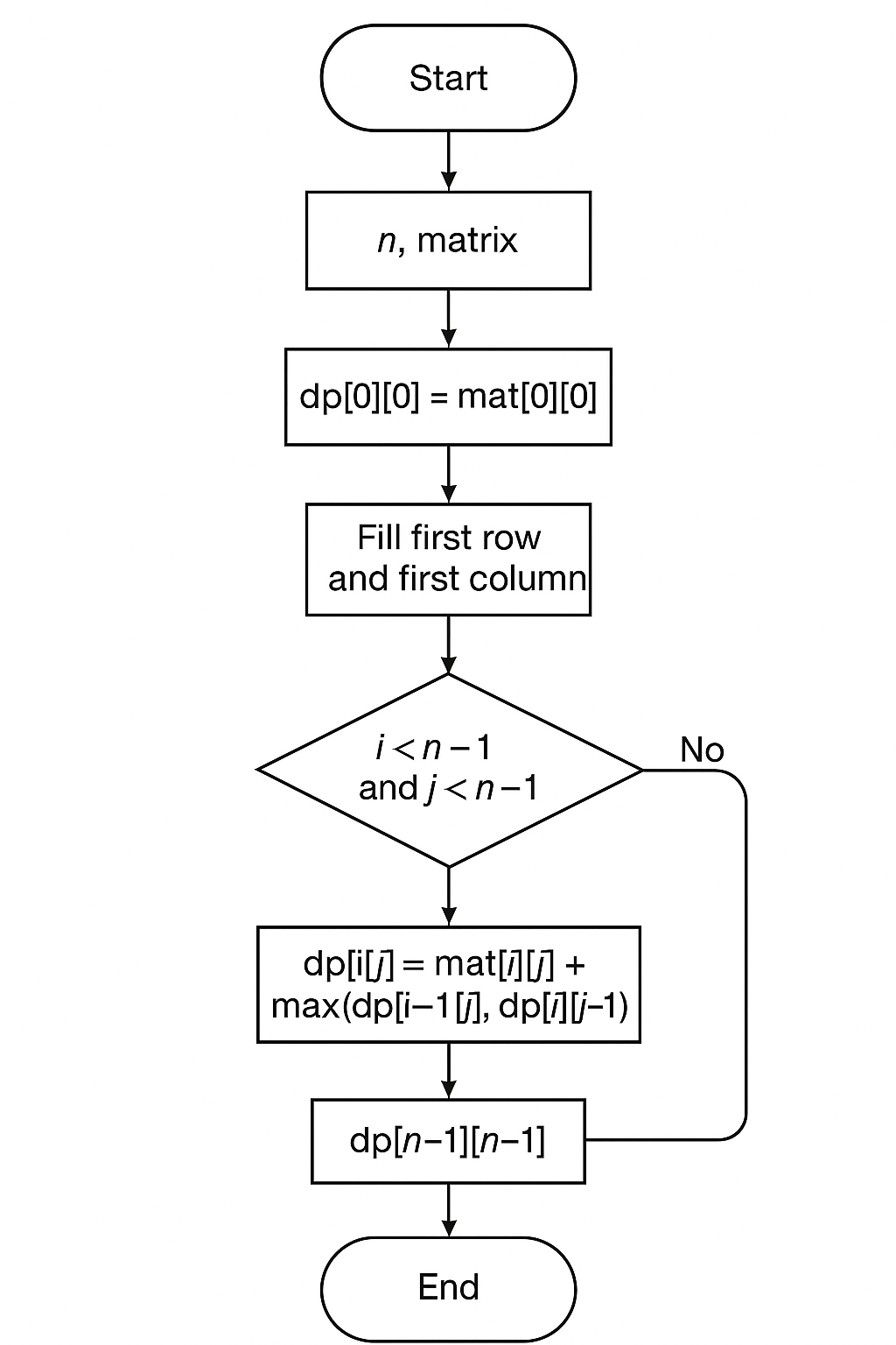
The main idea is to create a helper DP matrix dp[i][j] which, for every cell (i,j), stores the maximum sum of a path from the starting cell (0,0) to that cell. First the values for the starting cell, the first row and the first column are initialized. Then the remaining cells are filled iteratively using the formula dp[i][j] = mat[i][j] + max(dp[i-1][j], dp[i][j-1]). After the whole DP matrix is filled, the result is in dp[n-1][n-1].
Algorithm description (structure of the flowchart)
The algorithm can be shown in the following steps:
- Start: read the size
nand the matrixmat[n][n]. - Initialize the DP matrix:
- Set
dp[0][0] = mat[0][0]. - Fill the first row and the first column of the DP matrix.
- Set
- Main loop: for every cell
(i,j)where1 ≤ i,j ≤ n-1, computedp[i][j] = mat[i][j] + max(dp[i-1][j], dp[i][j-1]). - Result:
dp[n-1][n-1]contains the maximum path sum.
The flowchart of the algorithm is shown in Figure 1.
Solution 3 — Dynamic programming (Bottom-Up DP)
Try to think on your own how you would solve the problem without recursion, by gradually building optimal solutions from the start of the matrix. This is a classic example of dynamic programming.
In this approach we create a DP matrix dp[i][j] which stores the maximum sum from the starting cell (0,0) to cell (i,j).
The idea is that every cell is computed from previously computed values (above and to the left), which avoids recursion and repeated computation.
The complexity of this approach is O(n²) and it is the standard
optimal solution for this problem.
Previous
|<Preparation for the national competition and SIO (SR)