
Graphs — BFS and DFS (Basics)
What are graphs and trees used for in practice?
When we meet graphs and trees for the first time, a natural question comes up: what is this actually for, and where is it used in practice?
Graphs and trees are not abstract concepts that exist only in the theory of algorithms. On the contrary, they are one of the most often used models for describing real-world problems, especially when there are several objects connected with one another.
A tree is a special case of a graph that has a hierarchical structure. This means that there is one starting node (the root), and all the other nodes branch out from it, without cycles and without links back.
Trees are used when we want to represent relations of the kind: parent – child, superior – subordinate or general – specific.
Let us imagine the menu structure of a website:
- Home
- Algorithms
- Graphs
- BFS
- DFS
- Sorting
- Graphs
- Contact
This structure is a pure tree. Every page has its "parent", and the path to it is unique.
Exactly such structures are used in:
- website navigation
- menus in applications
- organising files and folders
We use a graph when the relations between objects are not strictly hierarchical. In other words, when objects can be connected in several ways.
Examples of problems that are naturally modelled with graphs are:
- a map of towns and the roads between them
- social networks (users and their friendships)
- computer networks
- dependencies between tasks
When we have a graph or a tree, we often want to answer questions like:
- Is there a path between two nodes?
- What is the shortest path?
- Which nodes can we reach?
- In what order should we visit them?
This is where the algorithms BFS and DFS come in.
BFS is especially useful when we are looking for:
- the shortest path (in the number of steps)
- solutions level by level
DFS is useful when we want:
- to explore one branch of a problem in detail
- to check whether there is a cycle
- to search through all possible solutions
In other words, graphs and trees let us translate real problems into a structure that algorithms can work on.
In the rest of the lesson we will see how BFS and DFS are applied to a concrete graph and why the same graph can give different traversal orders, depending on the algorithm we use.
A graph is a data structure made of nodes (vertices) and edges that connect those nodes. Graphs are used for modelling networks, roads, social connections, hierarchies and many real problems.
In algorithmics, knowing how to search graphs is the basis for more advanced topics: Dijkstra, MST algorithms, topological sorting, DP on graphs.
Representing a graph
The most common way in competitions is an adjacency list, because it is memory-efficient and allows fast processing.
vector<int> graph[100]; // for n nodes

// an example of adding an edge (an undirected graph):
graph[1].push_back(2);
graph[2].push_back(1);
Terminology:
- directed graph – the edges have a direction (A → B)
- undirected graph – the connections go both ways (A — B)
- weighted graph – every edge has a value (e.g. the length of a road)
- adjacency matrix – kept in the form of an n×n table (less practical)
To make it easier to understand the difference between the algorithms BFS (Breadth-First Search) and DFS (Depth-First Search), we will first define a concrete graph on which both algorithms will run.
The picture below shows a tree (a special case of a graph) with one starting node (the root) and several connected nodes. This graph will stay unchanged throughout the lesson — only the way the algorithms traverse it changes.
It is important to first see clearly the complete graph and all its connections, because this will help us later to follow, step by step, how BFS and DFS reach different traversal orders.
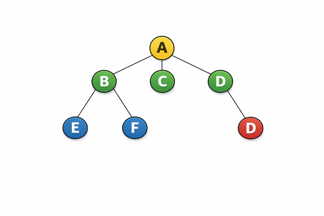
In the graph shown, node A is the starting node (the root of the tree). The nodes B, C and D branch out from it. Node B has further descendants E and F, while node D leads to node G.
We will use this graph as a reference from now on. No matter whether we apply BFS or DFS, the structure of the graph stays the same — the difference is only in the order in which the nodes are visited.
In the next picture we will see how this same graph is broken down step by step for both algorithms, with the traversal order and the flow of the search clearly marked.
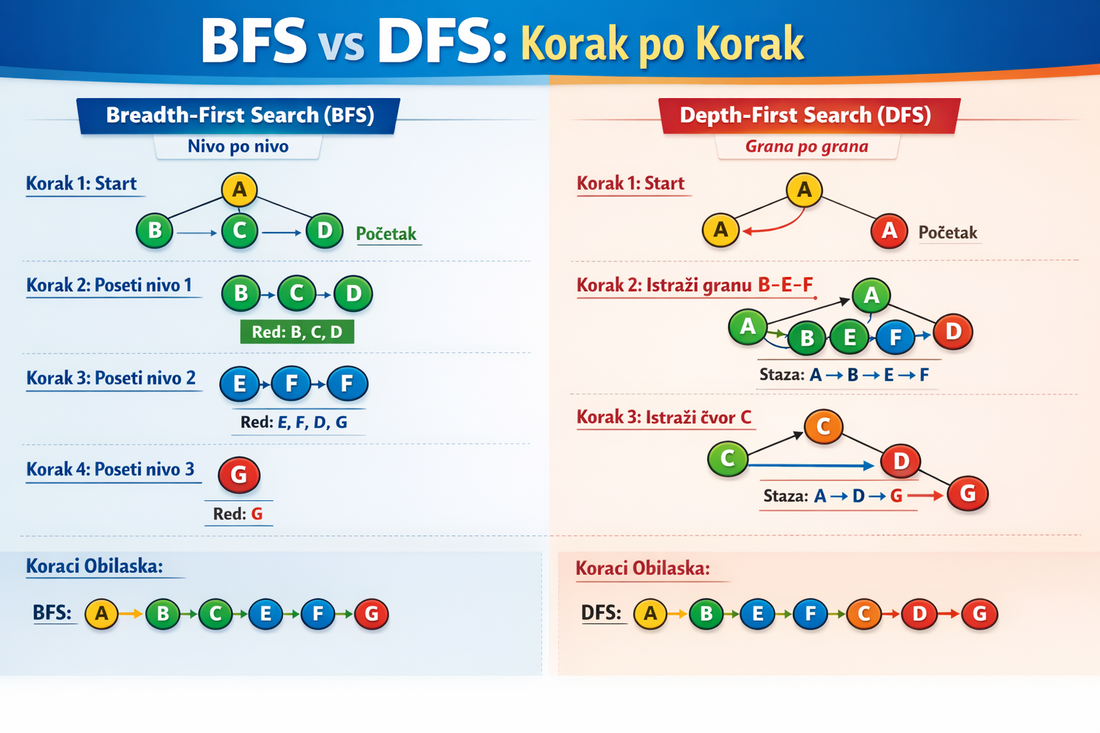
As the previous picture shows, BFS (breadth-first search) traverses the graph level by level. First all the nodes directly connected to the starting node are visited, and only then their descendants. This algorithm uses a queue to remember the nodes.
On the other hand, DFS (depth-first search) goes as deep as it can along one branch before it goes back and continues with the next branch. DFS is most often implemented with a stack or with recursion.
Exactly because of this difference in strategy, BFS and DFS give different traversal orders, even though they work on the same graph. Understanding this visualisation is the key to using these algorithms correctly in practice.
The adjacency matrix — another way to represent a graph
Besides an adjacency list, a graph can also be represented with an adjacency matrix.
That is a two-dimensional array adj[n][n] where:
adj[u][v] = 1if there is an edge between the nodes u and vadj[u][v] = 0if there is none
An example for an undirected graph with 4 nodes:
    0 1 2 3
0 [ 0 1 1 0 ]
1 [ 1 0 0 1 ]
2 [ 1 0 0 0 ]
3 [ 0 1 0 0 ]
When to use which representation?
| Adjacency list | Adjacency matrix |
|---|---|
| Efficient for sparse graphs (few edges) | Good for dense graphs |
| Memory: O(V + E) | Memory: O(V²) |
| Fast iteration through the neighbours | A fast check whether an edge exists (O(1)) |
In competitive programming the adjacency list is used most often, because graphs are usually large, but with relatively few edges.
BFS — Breadth-First Search
When and why to use BFS
We use the BFS (breadth-first search) algorithm when we want to explore the nodes of a graph by levels, i.e. first all the nodes closest to the starting one, then the next ones and so on. This property is crucial when we look for the shortest path (in terms of the number of edges) between two nodes of a graph, which is a common need in real problems.
For example, let us imagine a problem:
- In a maze we want to find the shortest path from the entrance to the exit.
- In a social network we want to find the smallest number of steps between two users (how many "friendships" separate them).
- In a computer network we explore which nodes are reachable in the minimum number of hops from the source node.
BFS traverses the graph by levels. First it visits all the neighbours of the starting node, then their neighbours, etc.
It is used for finding the shortest path in an unweighted graph.
The implementation uses a queue.
A visual explanation of BFS traversal
Breadth-First Search (BFS) traverses a graph by levels. This means that it first visits all the nodes 1 step away, then all the nodes 2 steps away, etc.
An example graph:
        0
      /   \
     1     2
    / \     \
   3   4     5
If we start from node 0, the traversal goes by levels:
- Level 0: 0
- Level 1: 1, 2
- Level 2: 3, 4, 5
0 → 1 → 2 → 3 → 4 → 5
That is why BFS guarantees that the first time we reach some node, we have reached it along the shortest path (by the number of edges).
Tracking the distances (the dist array)
To really find the shortest distance,
we use the array dist.
dist[i] = -1means that the node has not been visited yetdist[start] = 0because the starting node is 0 away from itself- For every neighbour:
dist[neighbour] = dist[v] + 1
Since BFS traverses the graph by levels,
the values in the dist array naturally grow level by level.
#include <bits/stdc++.h>
using namespace std;

vector<int> graph[100];
int dist[100];

void bfs(int start){
    queue<int> q;

    // Initialising the dist array
    for(int i = 0; i < 100; i++)
        dist[i] = -1;

    q.push(start);
    dist[start] = 0;

    while(!q.empty()){
        int v = q.front();
        q.pop();

        for(int neighbour : graph[v]){
            if(dist[neighbour] == -1){
                dist[neighbour] = dist[v] + 1;
                q.push(neighbour);
            }
        }
    }
}
A table of the states while BFS runs
The following table shows how the queue and the array of distances change while the algorithm runs on the example graph.
| Step | Node taken out | State of the queue | Dist array |
|---|---|---|---|
| Start | - | [0] | [0, -1, -1, -1, -1, -1] |
| 1 | 0 | [1, 2] | [0, 1, 1, -1, -1, -1] |
| 2 | 1 | [2, 3, 4] | [0, 1, 1, 2, 2, -1] |
| 3 | 2 | [3, 4, 5] | [0, 1, 1, 2, 2, 2] |
| 4 | 3 | [4, 5] | [0, 1, 1, 2, 2, 2] |
| 5 | 4 | [5] | [0, 1, 1, 2, 2, 2] |
| 6 | 5 | [] | [0, 1, 1, 2, 2, 2] |
We see that the values in the dist array grow level by level:
- Node 0 has the distance 0
- Nodes 1 and 2 have the distance 1
- Nodes 3, 4 and 5 have the distance 2
The first time we reach a node, we have already found its shortest distance from the starting node. That is the key property of the BFS algorithm.
An example of building the graph
int main(){
    graph[0] = {1, 2};
    graph[1] = {0, 3, 4};
    graph[2] = {0, 5};
    graph[3] = {1};
    graph[4] = {1};
    graph[5] = {2};

    bfs(0);
    return 0;
}
A visual animation — BFS step by step
Below is a detailed display of how BFS goes through the graph
level by level. We look at the graph from the previous example
and start BFS from node 0.
The structure of the graph
        0
       / \
      1   2
     / \   \
    3   4   5
A table of how the BFS algorithm runs
| Step | Node taken out | State of the queue | Dist array | Explanation |
|---|---|---|---|---|
| Start | - | [0] | [0, -1, -1, -1, -1, -1] | We put the starting node 0 into the queue and set dist[0] = 0. |
| 1 | 0 | [1, 2] | [0, 1, 1, -1, -1, -1] | We discover the neighbours 1 and 2. Their distance is 1. |
| 2 | 1 | [2, 3, 4] | [0, 1, 1, 2, 2, -1] | We discover 3 and 4. Their distance is 2. |
| 3 | 2 | [3, 4, 5] | [0, 1, 1, 2, 2, 2] | We discover 5. Its distance is 2. |
| 4 | 3 | [4, 5] | [0, 1, 1, 2, 2, 2] | No new nodes. |
| 5 | 4 | [5] | [0, 1, 1, 2, 2, 2] | No new nodes. |
| 6 | 5 | [] | [0, 1, 1, 2, 2, 2] | The queue is empty — BFS ends. |
An explanation by levels
Level 0: node 0
Level 1: nodes 1 and 2
Level 2: nodes 3, 4 and 5
BFS traverses the graph by levels because it uses a queue (a FIFO structure). This means that all the nodes at distance 1 are processed before the nodes at distance 2, and all the nodes at distance 2 before those at distance 3, etc.
Why is the distance found the shortest one?
When we reach some node for the first time, we have reached it with the smallest possible number of edges.
The reason is that BFS:
- First goes through all the shorter paths
- Then moves on to the longer ones
- Never comes back to a shorter path later
That is why BFS is the ideal algorithm for finding shortest paths in graphs without weights.
BFS with computing distances (the shortest path)
One of the most important uses of the BFS algorithm is finding the shortest distance from the starting node to all the other nodes in an unweighted graph.
We use the array dist, where:
dist[v]= the minimum number of edges from the starting node to the node v- At the start: we set all the values to -1 (the node has not been visited)
dist[start] = 0because the starting node is 0 away from itself
Since BFS traverses the graph by levels, the first time we reach a node we have guaranteed found its shortest distance.
#include <iostream>
#include <vector>
#include <queue>
using namespace std;

int main() {

    int n, m;
    cin >> n >> m;
    // n = the number of nodes in the graph
    // m = the number of edges

    // We create the adjacency list
    // adj[i] holds all the nodes connected to the node i
    vector<vector<int>> adj(n);

    // Reading all the edges of the graph
    for(int i = 0; i < m; i++) {
        int u, v;
        cin >> u >> v;
        // u and v are the nodes the edge connects

        adj[u].push_back(v);
        // we add v to the neighbour list of the node u

        adj[v].push_back(u);
        // we add u to the neighbour list of the node v
        // remove this line if the graph is directed
    }

    // the starting node from which we compute the distances
    int start = 0;
    // the nodes are assumed to be indexed from 0 to n-1

    // dist[i] keeps the shortest distance from start to i
    vector<int> dist(n, -1);
    // -1 means that the node has not been visited yet

    queue<int> q;
    // the queue we use in the BFS algorithm

    dist[start] = 0;
    // the distance of the starting node from itself is 0

    q.push(start);
    // we put the starting node into the queue

    // the BFS loop
    while(!q.empty()) {

        int u = q.front();
        // we take the node from the front of the queue

        q.pop();
        // we remove it from the queue

        // we go through all the neighbours of the node u
        for(int v : adj[u]) {

            // if the neighbour has not been visited yet
            if(dist[v] == -1) {

                // its distance is the distance of u + 1
                dist[v] = dist[u] + 1;

                // we add it to the queue so that later
                // we visit its neighbours too
                q.push(v);
            }
        }
    }

    // Printing the results
    // we show the shortest distance from start to every node
    for(int i = 0; i < n; i++) {
        cout << "Distance from "
             << start
             << " to "
             << i
             << " is "
             << dist[i]
             << endl;
    }

    return 0;
}
If some node is still equal to -1 after the algorithm has run,
it means that it is not reachable from the starting node (the graph is not fully connected).
A detailed explanation — BFS with computing distances
The BFS algorithm makes it possible to find the shortest distance from the starting node to all the other nodes in an unweighted graph.
Since all the edges have an implicit weight of 1, the shortest path means:
The path with the smallest number of edges.
What does the array dist represent?
We use the array dist[v], where:
dist[v]= the minimum number of edges from the starting node to the node v- At the start: all the values are
-1(the node has not been visited) dist[start] = 0
The value -1 means that we have not reached that node yet.
An example graph
        0
       / \
      1   2
     / \   \
    3   4   5
We start BFS from node 0.
A visual table of the execution
| Step | Node taken out | State of the queue | dist array | Level |
|---|---|---|---|---|
| Start | - | [0] | [0, -1, -1, -1, -1, -1] | 0 |
| 1 | 0 | [1, 2] | [0, 1, 1, -1, -1, -1] | 1 |
| 2 | 1 | [2, 3, 4] | [0, 1, 1, 2, 2, -1] | 2 |
| 3 | 2 | [3, 4, 5] | [0, 1, 1, 2, 2, 2] | 2 |
| 4 | 3 | [4, 5] | [0, 1, 1, 2, 2, 2] | -- |
| 5 | 4 | [5] | [0, 1, 1, 2, 2, 2] | -- |
| 6 | 5 | [] | [0, 1, 1, 2, 2, 2] | -- |
What do we notice?
- Level 0 → node 0
- Level 1 → nodes 1 and 2
- Level 2 → nodes 3, 4 and 5
BFS traverses the graph by levels because it uses a queue (FIFO). First all the nodes at distance 1 are processed, then all the nodes at distance 2, etc.
Why is the first arrival at a node the shortest path?
When we reach the node v for the first time:
dist[v] = dist[u] + 1This means that we reached it along the shortest possible path, because BFS never skips levels.
There is no way to find a shorter path later, since it would have to have fewer edges, and all the shorter paths have already been processed earlier.
An important note
If after the algorithm ends:
dist[i] == -1it means that node i is not reachable from the starting node.
Time complexity
For a graph represented with an adjacency list:
O(n + m)
- n — the number of nodes
- m — the number of edges
- m — the number of edges
The key property of the BFS algorithm
The first time we reach a node, we have already found its shortest distance.
This property holds only for unweighted graphs.
BFS on a grid (the maze problem)
A graph does not always have to be given explicitly. In problems with a matrix (e.g. a maze), we can look at every cell as a node, and moving to a neighbouring cell as an edge.
The allowed moves are: up, down, left and right. Every move is one edge (one step).
If a cell is marked with the character '.', we consider it passable.
Other characters (e.g. '#') can be walls.
#include <iostream>
#include <queue>
using namespace std;

// The arrays are global: a matrix of 1000 × 1000 is too big
// for the local variables of main (stack overflow).
char grid[1000][1000];
// the matrix that represents the maze

int dist[1000][1000];
// dist[i][j] = the minimum number of steps
// from the starting cell to the cell (i,j)

int main() {

    int n, m;
    cin >> n >> m;
    // n = the number of rows of the matrix
    // m = the number of columns of the matrix

    // Reading the matrix and initialising the dist array
    for(int i = 0; i < n; i++) {
        for(int j = 0; j < m; j++) {
            cin >> grid[i][j];
            // we read the character that represents the cell

            dist[i][j] = -1;
            // -1 means that the cell has not been visited yet
        }
    }

    // BFS uses a queue
    queue<pair<int,int>> q;

    // the starting position in the maze
    int startX = 0;
    int startY = 0;

    // the starting cell has the distance 0
    dist[startX][startY] = 0;

    // we put the starting cell into the queue
    q.push({startX, startY});

    // Moves in the 4 directions
    // index 0 → down
    // index 1 → up
    // index 2 → right
    // index 3 → left
    int dx[4] = {1, -1, 0, 0};
    int dy[4] = {0, 0, 1, -1};

    // The main BFS loop
    while(!q.empty()) {

        // we take the current cell from the queue
        auto [x, y] = q.front();
        // a C++17 structured binding:
        // x = row, y = column

        q.pop();

        // we check all 4 neighbouring cells
        for(int d = 0; d < 4; d++) {

            int nx = x + dx[d];
            int ny = y + dy[d];
            // nx, ny are the new cell

            // Checking whether we are inside the borders of the matrix
            if(nx >= 0 && nx < n && ny >= 0 && ny < m) {

                // If the cell is passable and has not been visited
                if(grid[nx][ny] == '.' && dist[nx][ny] == -1) {

                    // the distance is +1 step from the current cell
                    dist[nx][ny] = dist[x][y] + 1;

                    // we put the new cell into the queue
                    // so that we explore its neighbours later
                    q.push({nx, ny});
                }
            }
        }
    }

    return 0;
}
Since BFS goes through the cells by levels,
dist[i][j] is the minimum number of steps
needed to reach that cell from the starting position.
If some cell stays equal to -1,
it means that it cannot be reached.
BFS on a grid is ideal for problems about the minimum number of steps. If a problem asks you to optimise a sum (e.g. the minimum sum of weights), dynamic programming or Dijkstra's algorithm is a better choice.
If you are interested in optimising a path through a grid (e.g. minimising a sum) instead of just the number of steps, see also Grid DP — dynamic programming on a matrix .
A visual example of a BFS search in a maze
Let us look at the following simple maze.
The cell S is the starting position,
. are passable cells, and # are walls.
S . . #
# . . #
# . . .
# # . E
The goal is to find the minimum number of steps from the starting cell S
to every reachable cell in the maze.
After the BFS algorithm has run, the matrix of distances can look like this:
0 1 2 X
X 2 3 X
X 3 4 5
X X 5 6
0marks the starting cell- every number is the minimum number of steps from the starting position
Xmarks a wall or an unreachable cell
BFS goes through the cells by levels:
- first all the cells 1 step away
- then all the cells 2 steps away
- then all the cells 3 steps away, etc.
That is why BFS always finds the shortest path in graphs without weights, which makes it the ideal algorithm for maze and grid problems.
Comparing BFS and DFS
Although both algorithms are used to traverse a graph, the way they work and their uses are different.
| Property | BFS | DFS |
|---|---|---|
| Data structure | Queue | Stack / recursion |
| Way of traversal | By levels | In depth (goes as deep as possible) |
| Shortest path (unweighted graph) | Yes | Not guaranteed |
| Typical use | Shortest path, minimum number of steps | Connected components, cycles |
| Memory | Can use more (keeps a level) | Usually less |
Intuitively:
- BFS explores the "width" of the graph.
- DFS explores the "depth" of the graph.
If your goal is the minimum number of steps — use BFS.
If your goal is to visit all the components or check for cycles — DFS is often the more natural choice.
DFS — Depth-First Search
When and why to use DFS
The DFS (depth-first search) algorithm uses the strategy of exploring one direction in the graph "to the end" before it goes back and explores other directions. This approach is especially useful when we want to:
- check whether there is a path between nodes at all;
- determine whether a graph contains a cycle;
- find all the nodes that are part of the same connected component;
- perform a topological sort when we work with directed acyclic graphs.
- in a maze search problem, DFS can explore one path to the end and go back if it was a "dead end";
- in a system of tasks with dependencies (e.g. compiling modules), DFS is used to determine the order in which the tasks can be done without breaking the dependencies.
A step-by-step DFS simulation
We use the same graph as in the BFS example:
        0
      /   \
     1     2
    / \     \
   3   4     5
DFS goes as deep as possible before it goes back. Let us assume that we visit the neighbours in the order in which they are listed.
Start
We start from node 0.
Step 1
0 → we move to 1 (the first neighbour)
Step 2
1 → we move to 3
Step 3
3 has no new neighbours → we go back to 1
Step 4
From 1 we move to 4
Step 5
4 has no new neighbours → we go back to 1 → then to 0
Step 6
From 0 we move to 2
Step 7
2 → we move to 5
A possible traversal order:
0 → 1 → 3 → 4 → 2 → 5
We see that DFS goes deep through one branch before it goes back. Unlike BFS, it does not visit the nodes by levels.
DFS goes as deep as possible into the graph until it reaches the end, and then it goes back (backtracking) and continues the search from the previous node. The most common implementation of the DFS algorithm uses recursion, which means that the function calls itself for the neighbouring nodes.
DFS is often used for:
- checking whether a graph is connected
- finding cycles
- topological sorting (directed graphs)
- finding connected components
- searching mazes, trees and other structures
// Including all the standard C++ libraries
#include <bits/stdc++.h>
using namespace std;

// The adjacency list of the graph
// graph2[i] holds all the nodes connected to the node i
vector<int> graph2[100];

// The array that marks whether a node has already been visited
// true  → the node has already been processed
// false → the node has not been visited yet
bool visited[100];

// The DFS function that traverses the graph starting from the node v
void dfs(int v){

    // We mark the current node as visited
    visited[v] = true;

    // We print the current node
    cout << v << " ";

    // We go through all the neighbours of the node v
    for(int neighbour : graph2[v]){

        // If the neighbour has not been visited yet
        // we call DFS recursively for that node
        if(!visited[neighbour])
            dfs(neighbour);
    }
}
Calling the function:
int main(){

    // Building an undirected graph by hand
    // Every node has a list of its neighbours
    graph2[1] = {2, 3, 4};
    graph2[2] = {1, 3};
    graph2[3] = {1, 2, 4};
    graph2[4] = {1, 3};

    // Starting the DFS algorithm from node 1
    // DFS will traverse the graph as deep as possible
    dfs(1);

    return 0;
}
Output:
1 2 3 4 BFS vs DFS — a comparison
| Property | BFS | DFS |
|---|---|---|
| Data structure | Queue | Recursion or a stack |
| Search order | Level by level (the width of the graph) | Goes as deep as possible, then goes back |
| Shortest path? | YES (if the graph has no weights) | NO |
| Time complexity | O(V + E) | O(V + E) |
| Example uses | Shortest path, breadth search | Topological sorting, cycles, components |
Exercises and tasks
Try the following tasks:
- Compute the distance (the number of steps) of every node from the starting one using BFS.
- Count how many nodes there are in a connected component using DFS.
- Determine whether a graph is connected.
- Write a program that checks whether there is a cycle in an undirected graph.
This knowledge is the basis for the next topics, such as: Dijkstra's algorithm, MST (Kruskal and Prim) and topological sorting.
Detecting a cycle with DFS
One of the important uses of the DFS algorithm is detecting a cycle in a graph.
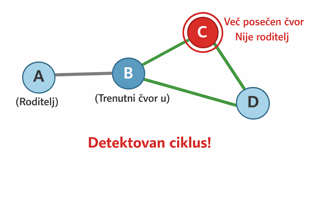
In an undirected graph a cycle exists if during the DFS traversal we come across an already visited node that is not the parent of the current node.
#include <iostream>
#include <vector>
using namespace std;

// The adjacency list of the graph
// adj[i] holds all the nodes connected to the node i
vector<vector<int>> adj;

// The array that marks whether a node has already been visited
vector<bool> visited;

// The variable that marks whether the graph contains a cycle
bool hasCycle = false;

// The DFS function
// u      - the current node
// parent - the node from which we came to the current node
void dfs(int u, int parent) {

    // We mark the current node as visited
    visited[u] = true;

    // We go through all the neighbours of the node u
    for(int v : adj[u]) {

        // If the neighbour has not been visited yet
        // we continue the DFS traversal
        if(!visited[v]) {
            dfs(v, u);
        }

        // If the neighbour has already been visited
        // and is not the parent of the current node,
        // then there is a cycle in the graph
        else if(v != parent) {
            hasCycle = true;
        }
    }
}

int main() {

    int n, m;
    // n - the number of nodes
    // m - the number of edges

    cin >> n >> m;

    // We create the adjacency list for n nodes
    adj.resize(n);

    // We initialise the array visited to false
    visited.assign(n, false);

    // Reading the edges of the graph
    for(int i = 0; i < m; i++) {

        int u, v;

        // we read the ends of the edge
        cin >> u >> v;

        // Since the graph is undirected,
        // we add the edge in both directions
        adj[u].push_back(v);
        adj[v].push_back(u);
    }

    // We start DFS from every node
    // (needed if the graph is not connected)
    for(int i = 0; i < n; i++) {
        if(!visited[i])
            dfs(i, -1);
    }

    // Printing the result
    if(hasCycle)
        cout << "The graph contains a cycle\n";
    else
        cout << "The graph has no cycle\n";
}
In an undirected graph we must ignore the edge to the parent, because it does not form a cycle. When during the DFS traversal we come across an already visited node that is not the parent of the current node, it means that there is another path to that node, and so a cycle has been formed in the graph.
Practice tasks — BFS and DFS
1. BFS — the shortest distance from the starting node
Task text
An undirected graph with n nodes is given.
Using the BFS algorithm, compute
the shortest distance (the number of edges) from the starting node
s to all the other nodes in the graph.
Example
Input:
Graph:
1 - 2
1 - 3
2 - 4
3 - 4
Start = 1

Output:
dist[1] = 0
dist[2] = 1
dist[3] = 1
dist[4] = 22. BFS — checking whether a graph is connected
Task text
An undirected graph is given. Check whether the graph is connected.
3. DFS — the number of nodes in a connected component
Task text
An undirected graph and a starting node s are given.
Using the DFS algorithm, compute how many nodes belong to
the connected component that contains the node s.
Example
Input:
Graph:
1 - 2
2 - 3
4 - 5
Start = 1

Output:
Number of nodes in the component = 3
4. DFS — detecting a cycle in an undirected graph
Task text
An undirected graph is given. Determine whether the graph contains a cycle using the DFS algorithm.
Example
Input:
Graph:
1 - 2
2 - 3
3 - 1

Output:
The graph CONTAINS a cycle
Practical tasks (real problems) — BFS and DFS
5. The shortest route in a network of city roads (BFS)
Task text
A city is represented as an unweighted graph in which the nodes are crossroads,
and the edges are two-way roads between them.
N crossroads and a list of roads are given.
Find the smallest number of roads you need to travel
to get from the crossroads S to the crossroads T.
Example
Input:
5 6
1 2
1 3
2 4
3 4
4 5
2 5
S = 1, T = 5

Output:
2

Explanation:
The shortest route is 1 → 2 → 5 (two edges).
6. Evacuating an area – checking connectivity (DFS)
Task text
During a natural disaster, an area is divided into zones.
The zones are connected by passages and represented as a graph.
Check whether all the zones are reachable
from the command centre (zone 1).
If some zone is not reachable, the evacuation is not possible.
Example
Input:
6 4
1 2
2 3
3 4
5 6

Output:
NO

Explanation:
Zones 5 and 6 are not connected to zone 1.
Medium-difficulty tasks — BFS and DFS
7. BFS — reconstructing the shortest path (the parent array)
Task text
An undirected graph and two nodes s and t are given.
Using the BFS algorithm, find
the shortest path from the node s to the node t
and print all the nodes on that path.
Example
Input:
Graph:
1 - 2
1 - 3
2 - 4
3 - 4
Start = 1
End = 4

Output:
1 2 4
8. DFS — the number of connected components
Task text
An undirected graph with n nodes is given.
Using the DFS algorithm, compute
the number of connected components in the graph.
Example
Input:
Graph:
1 - 2
2 - 3
4 - 5

Output:
Number of components = 2
Check your knowledge
Open the quiz
BFS and DFS
1. Which structure is used in BFS traversal?
2. What does BFS find in a graph in which all the edges have the same length?
3. What is the complexity of BFS and DFS with an adjacency list?
4. How are connected components counted?