
SCC — Strongly Connected Components (Kosaraju and Tarjan)
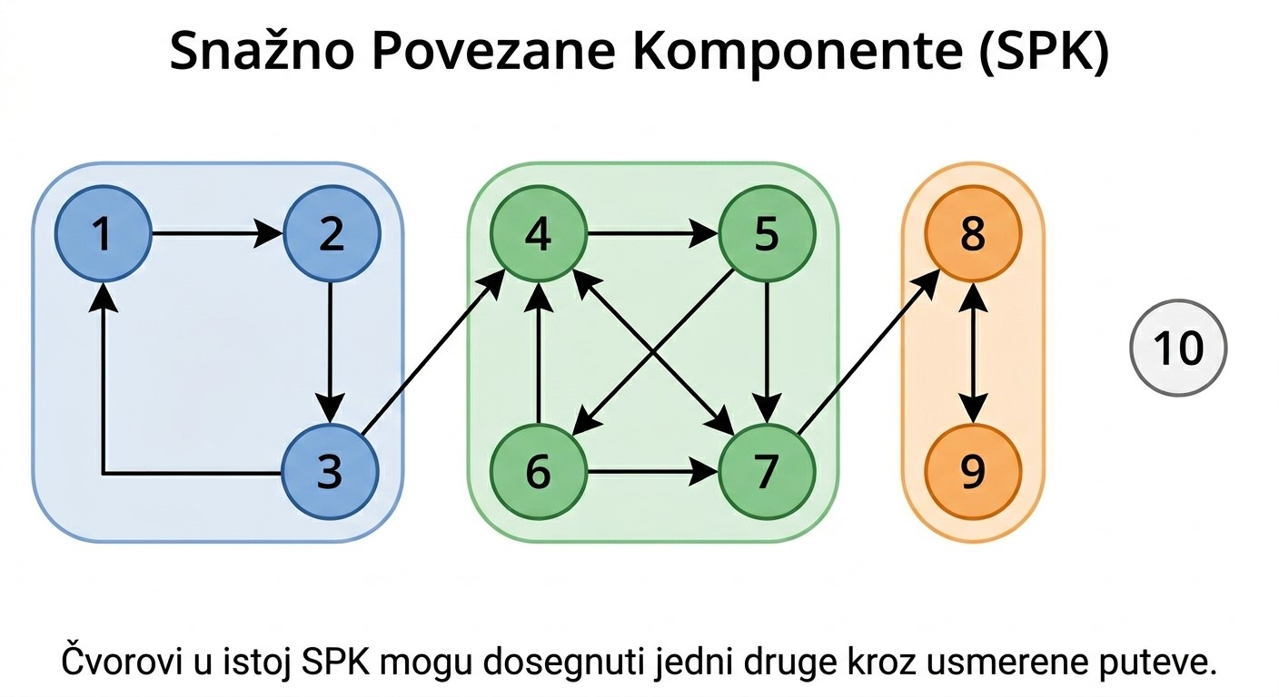
Strongly connected components (SCC) are a key concept for analysing directed graphs.
An SCC is a subset of vertices in which every vertex can be reached from every other one. This means that for vertices in the same SCC the following holds:
u → v and v → u (there are paths in both directions)
This structure is especially important in:
- compilers (dependency analysis)
- professional systems (tariffs, networks, data streams)
- game theory and state graphs
- web graphs (PageRank, network fragmentation)
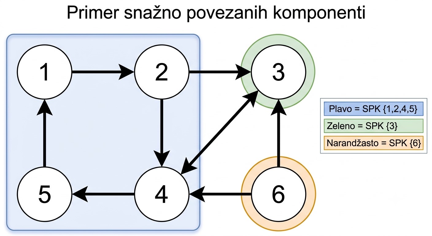
An example graph
   (1) → (2) → (3)
    ↑     ↓      ↑
    |     ↑      |
    |     |      |
   (5) ← (4) ← (6)
The edges in the graph:
1 → 2
2 → 3
2 → 4
4 → 2
4 → 5
5 → 1
6 → 4
6 → 3
The SCC (Strongly Connected Components) groups are:
- {1,2,4,5}
- {3}
- {6}
At first glance it may seem that it is enough for vertices to form a cycle in order to make an SCC, but the definition is stricter.
A strongly connected component is a maximal set of vertices such that for every two vertices u and v from that set there are paths in both directions:
u → v

and

v → u
The word maximal means that we cannot add any new vertex to that group and still have all the vertices reachable from one another.
In this example the vertices:
1 → 2 → 4 → 5 → 1
form a cycle, but that is not the only reason why they are in the same SCC. What matters is that from each of these vertices we can reach every other one and come back. That is why together they form one strong component:
{1,2,4,5}
Why is vertex 3 not in that group?
We can reach vertex 3, for example, through:
2 → 3
but from vertex 3 there is no path back to the vertices 1, 2, 4 or 5. That is why vertex 3 must stay in a separate SCC:
{3}
Similarly, vertex 6 also cannot be returned to from any other vertex. Although from it we can reach:
6 → 4
6 → 3
there is no path along which we could return to 6 from the other vertices. That is why it is a separate SCC too:
{6}
It is important to point out that an SCC is not the same as an ordinary cycle.
For example, the set:
{1,2}
is not an SCC, although 1 and 2 are part of a larger cycle. The reason is that we can add more vertices, such as 4 and 5, and it would still hold that all of them can reach one another. That is why an SCC must be the largest possible such set.
In other words, an SCC is the largest group of vertices in which every vertex can reach every other vertex and come back.
Kosaraju's algorithm — the idea
Let us look at the graph from the previous example:
   (1) → (2) → (3)
    ↑     ↓      ↑
    |     ↑      |
    |     |      |
   (5) ← (4) ← (6)
Its SCCs are:
{1,2,4,5}
{3}
{6}
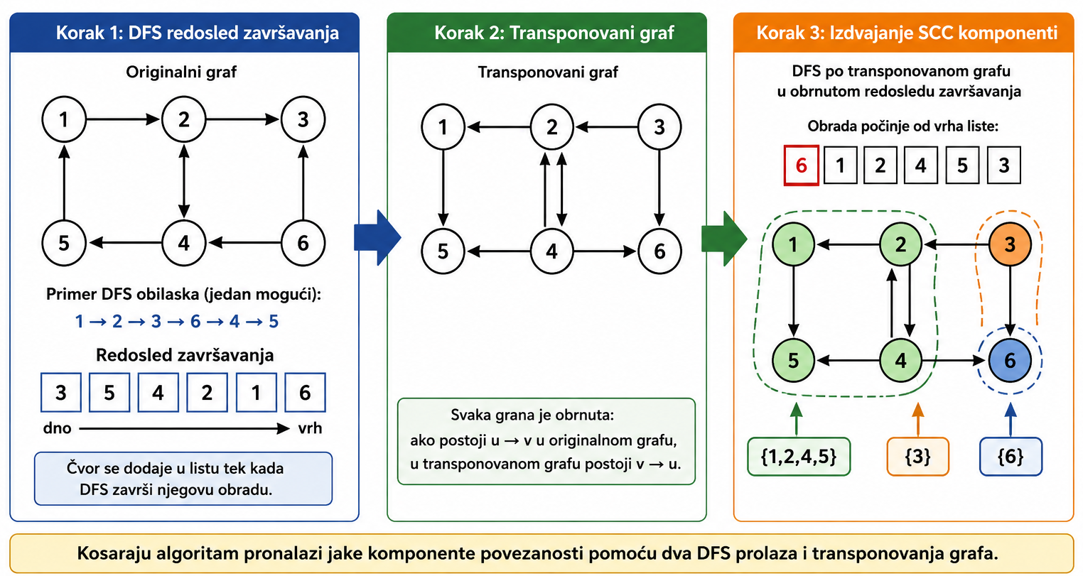
Kosaraju's algorithm finds these components using two DFS passes:
- DFS on the original graph, recording the order in which the vertices finish
- Transposing (reversing) all the edges
- DFS on the transposed graph in the reverse finishing order
The key idea of the algorithm is not just DFS, but exactly the order in which the vertices are processed in the second pass.
In the first DFS a vertex is not added to the list order when we visit it for the first time, but only when we have finished processing all its neighbours. That is why the list order is the DFS finishing order.
One possible run of the first DFS pass
DFS starts from vertex 1:

1 → 2 → 3

Vertex 3 has no unvisited neighbours,
so it finishes first.

We go back to 2.

2 → 4 → 5

Vertex 5 finishes.
Then 4 finishes.
Then 2 finishes.
Then 1 finishes.

Vertex 6 has not been visited yet,
so we start a new DFS from 6.
One possible finishing order is:
order = [3,5,4,2,1,6]
Note: the exact DFS order can depend on the order of the neighbours in the adjacency list, but the principle of the algorithm stays the same.
In the second pass we process the vertices in reverse order:
reversed(order)

[6,1,2,4,5,3]
Before the second DFS we build the transposed graph.
If the original graph had the edge:
u → v
in the transposed graph it becomes:
v → u
So the directions of all the edges are reversed.
Why is this useful?
If we look at every SCC as one "super-vertex", we get a graph called the SCC DAG. That graph has no cycles.
The first DFS gives us the order in which to start in the second pass. When in the transposed graph we start from the first unvisited vertex in reversed(order), the DFS stays inside one SCC and does not spill over into other components.
For our example, one possible order of extracting the components is:
{6}
{1,2,4,5}
{3}
In the end we get the same SCC groups:
{1,2,4,5}
{3}
{6}
It is important to point out that the order in which the SCCs are printed does not matter. What matters is only that the components are extracted correctly. The algorithm may first print {6}, then {1,2,4,5}, then {3}, or some other order, depending on the traversal order.
This is exactly why Kosaraju uses two DFS passes: the first determines the correct processing order, and the second extracts one SCC at a time in the transposed graph.
Kosaraju — a C++ implementation
#include <iostream>
#include <vector>
#include <algorithm>
using namespace std;

// ------------------------------------------------------------
// g  = the original directed graph
// gt = the transposed graph
//
// If the original graph has:
//
// u → v
//
// then the transposed one has:
//
// v → u
// ------------------------------------------------------------

vector<vector<int>> g, gt;

// ------------------------------------------------------------
// used[v]
// = whether the vertex has already been visited during DFS
// ------------------------------------------------------------

vector<bool> used;

// ------------------------------------------------------------
// order
// keeps the DFS finishing order
//
// A vertex is added ONLY when DFS finishes processing it.
//
// This is the key idea of Kosaraju's algorithm.
// ------------------------------------------------------------

vector<int> order;

// ------------------------------------------------------------
// comp
// the current SCC
// ------------------------------------------------------------

vector<int> comp;


// ============================================================
// THE FIRST DFS
// ============================================================
//
// DFS on the ORIGINAL graph.
//
// Goal:
// determine the finishing order of the vertices.
//
// When we finish processing a vertex,
// we add it to the vector "order".
//
// Vertices that finish later
// will be processed earlier in the second DFS.
// ============================================================

void dfs1(int v){

    // we mark the vertex as visited
    used[v] = true;

    // we go through all the neighbours
    for(int to : g[v]){

        // DFS only if the neighbour has not been visited
        if(!used[to])
            dfs1(to);
    }

    // --------------------------------------------------------
    // THIS IS THE MOST IMPORTANT PART
    // --------------------------------------------------------
    //
    // We add the vertex ONLY after its DFS has finished.
    //
    // This means:
    //
    // all the vertices reachable from v
    // have already been processed.
    //
    // That is why order represents:
    //
    // "the order of leaving the DFS"
    // --------------------------------------------------------

    order.push_back(v);
}


// ============================================================
// THE SECOND DFS
// ============================================================
//
// DFS on the TRANSPOSED graph.
//
// When we start from the right vertex,
// we will visit exactly one SCC.
//
// We add all the visited vertices to "comp".
// ============================================================

void dfs2(int v){

    used[v] = true;

    // we add the vertex to the current SCC
    comp.push_back(v);

    // DFS on the transposed graph
    for(int to : gt[v]){

        if(!used[to])
            dfs2(to);
    }
}


int main(){

    ios::sync_with_stdio(false);
    cin.tie(nullptr);

    int n, m;
    cin >> n >> m;

    // --------------------------------------------------------
    // We create graphs of size n
    // --------------------------------------------------------

    g.assign(n, {});
    gt.assign(n, {});
    used.assign(n, false);

    // --------------------------------------------------------
    // Reading the edges
    // --------------------------------------------------------
    //
    // The input:
    //
    // a b
    //
    // means:
    //
    // a → b
    //
    // In the transposed graph:
    //
    // b → a
    // --------------------------------------------------------

    for(int i = 0; i < m; i++){

        int a, b;
        cin >> a >> b;

        // switching to 0-based indexing
        --a;
        --b;

        // the original graph
        g[a].push_back(b);

        // the transposed graph
        gt[b].push_back(a);
    }


    // ========================================================
    // THE FIRST DFS
    // ========================================================
    //
    // We run DFS from all the unconnected components.
    //
    // Goal:
    // fill the vector "order".
    // ========================================================

    for(int i = 0; i < n; i++){

        if(!used[i])
            dfs1(i);
    }


    // ========================================================
    // RESETTING the visited array
    // ========================================================

    fill(used.begin(), used.end(), false);


    // ========================================================
    // THE SECOND DFS
    // ========================================================
    //
    // We process the vertices:
    //
    // in the reverse order from "order"
    //
    // Why?
    //
    // The SCC DAG has the property that
    // "source" components finish later.
    //
    // By processing from the end we guarantee
    // that every DFS catches exactly one SCC.
    // ========================================================

    for(int i = n - 1; i >= 0; i--){

        int v = order[i];

        // if the vertex has not been visited,
        // we find a new SCC
        if(!used[v]){

            // we empty the current component
            comp.clear();

            // DFS on the transposed graph
            dfs2(v);

            // ------------------------------------------------
            // Printing the SCC
            // ------------------------------------------------

            cout << "SCC: ";

            for(int x : comp)
                cout << x + 1 << " ";

            cout << "\n";
        }
    }
}
Example (the graph from the lesson)
Input
6 8
1 2
2 3
2 4
4 2
4 5
5 1
6 4
6 3
Output
SCC: 6
SCC: 1 5 4 2
SCC: 3
If we look at the list order as a stack, the vertex that finishes its DFS last will be at the top of the stack.
order = [3,5,4,2,1,6]

Top of the stack
    6
    1
    2
    4
    5
    3
Bottom of the stack
Kosaraju — a Python variant
from collections import defaultdict

g  = defaultdict(list)
gt = defaultdict(list)
order = []
visited = set()

def dfs1(v):
    visited.add(v)
    for to in g[v]:
        if to not in visited:
            dfs1(to)
    order.append(v)

def dfs2(v, comp):
    visited.add(v)
    comp.append(v)
    for to in gt[v]:
        if to not in visited:
            dfs2(to, comp)

n, m = map(int, input().split())
for _ in range(m):
    a, b = map(int, input().split())
    g[a].append(b)
    gt[b].append(a)

for i in range(1, n+1):
    if i not in visited:
        dfs1(i)

visited.clear()

for v in reversed(order):
    if v not in visited:
        comp = []
        dfs2(v, comp)
        print("SCC:", comp)
For the same input the Python program prints SCC: [6], SCC: [1, 5, 4, 2] and SCC: [3].
Tarjan's algorithm — one DFS
Tarjan is more efficient: it uses one DFS and low-link values, similar to finding bridges and articulation points.
It keeps a stack of the vertices that are currently active in the search. When the root of an SCC is found, it pops all the elements of that component from the stack.
vector<int> tin, low, st;
vector<bool> onStack;
int timer = 0;

void dfs_tarjan(int v){
    tin[v] = low[v] = ++timer;
    st.push_back(v);
    onStack[v] = true;

    for(int to : g[v]){
        if(!tin[to]){
            dfs_tarjan(to);
            low[v] = min(low[v], low[to]);
        }
        else if(onStack[to]){
            low[v] = min(low[v], tin[to]);
        }
    }

    if(tin[v] == low[v]){
        cout << "SCC: ";
        while(true){
            int node = st.back(); st.pop_back();
            onStack[node] = false;
            cout << node+1 << " ";
            if(node == v) break;
        }
        cout << "\n";
    }
}
Visualising Tarjan's algorithm (low-link)
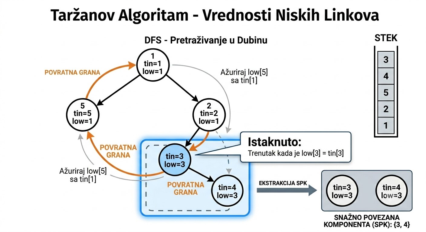
The run of Tarjan's algorithm on the graph from this lesson (DFS starts from vertex 1, the neighbours are visited in the order of the input edges):
vertex:  1  2  3  4  5  6
tin:     1  2  3  4  5  6
low:     1  1  3  1  1  6

1 → 2 → 3      3 has no outgoing edges: low[3] == tin[3] → SCC {3}
2 → 4 → 5      4 → 2 is on the stack: low[4] = 2
               5 → 1 is on the stack: low[5] = 1, then low[4] = 1, low[2] = 1
back to 1      low[1] == tin[1], stack [1, 2, 4, 5] → SCC {5, 4, 2, 1}
6              its edges go to vertices that are no longer on the stack → SCC {6}
A vertex stays on the stack until its whole component is closed: the values low come back to the DFS parents that are part of the cycle, and the component is popped only at the vertex for which low[v] == tin[v].
Why are SCCs important in competitive programming?
At first glance an SCC may look like "just another graph algorithm". However, strongly connected components are one of the most important techniques in advanced competitive programming.
The main idea is:
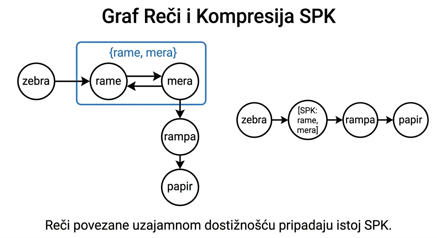
This is extremely important because many problems are much easier to solve on DAGs than on general directed graphs.
Intuition
If it is possible to move in both directions between several vertices, then they practically form one "whole".
For example:
A → B → C
↑       ↓
└───────┘
From every vertex we can reach every other one, so all three vertices belong to the same SCC.
Instead of looking at:
A, B, C
we can "collapse" them into one super-vertex:
[SCC]
The condensation graph
When we replace every SCC with one vertex, we get a new graph called the:
condensation graph
The most important property:
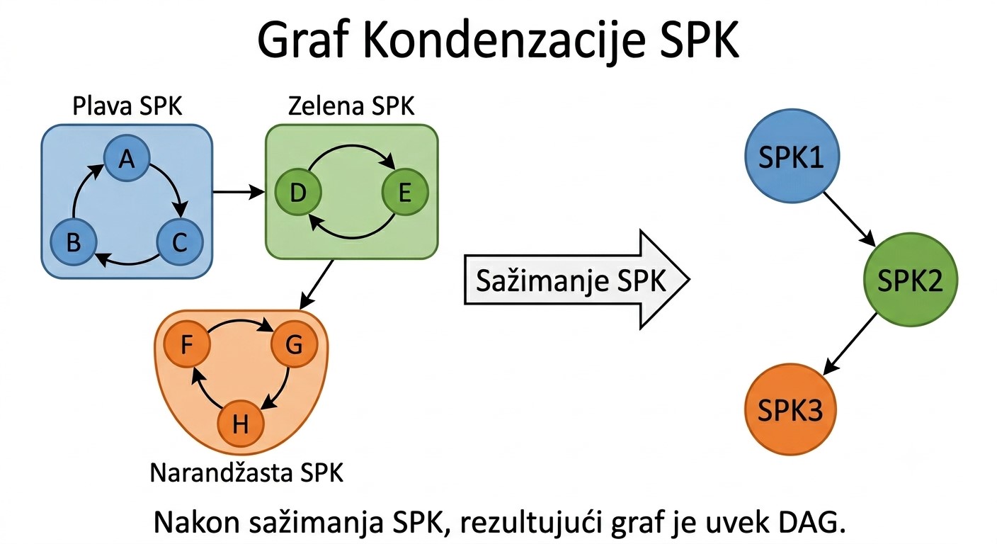
Why?
If there were a cycle between SCCs, then all those components would actually form one larger SCC.
Why is this useful?
When we get a DAG:
- we can do topological sorting
- we can use DP on the graph
- we can count the number of paths
- we can look for the longest paths
- we can propagate information between components
That is why SCC often appears as:
1. find the SCCs
2. collapse the graph
3. do DP on the DAG
The connection with real competition tasks
Many hard problems actually have hidden cycles that complicate the solution.
SCC makes it possible to:
- eliminate cycles
- group mutually dependent states
- simplify the graph
- move on to a much easier DAG problem
SCC + DAG + DP
An example of a typical task
Imagine a graph of words:
"zebra"   → "range"
"range"   → "gerbera"
"gerbera" → "rapid"
"rapid"   → "idol"
If it is possible to return between some groups of words, those words form an SCC.
After collapsing the SCCs, the problem often comes down to:
- how many vertices we can reach
- what the maximum profit is
- how many paths there are
- what the longest chain is
That is exactly why SCC is one of the foundations of advanced graph algorithms.
A typical progression of knowledge
DFS/BFS
   ↓
Topological sorting
   ↓
DAG DP
   ↓
SCC
   ↓
SCC + DAG + DP
When a student understands SCC, a large number of serious competition problems opens up.
Practice tasks
- Determine the SCCs in a graph that represents the dependencies of modules in software.
- Apply SCC to detect circular references in databases.
- Determine how many SCCs there are and what their representatives are.
- Write a program that reduces a graph to the DAG of its SCCs.
Tasks to solve on your own
Task 1: Kaladont — the number of reachable words
In the game kaladont (a word chain game) a sequence of words is formed so that the final syllable of the previous word matches the initial syllable of the next word.
In this task, the initial syllable is defined as the first two characters of the word, and the final syllable as the last two characters.
A dictionary containing N different words (lowercase English letters) is given. For every word, determine how many different words from the dictionary can be reached if that word is the starting one.
In other words, for every starting word count how many words there are for which there is at least one valid kaladont sequence that starts with that word and in which that word appears.
Input: the number N, and then N words. Output: for every word, in the order of the input, the number of reachable words (the starting word included).
Example
Input
5
zebra
range
gerbera
rapid
idol
Output
5
4
4
2
1
From zebra (ends with "ra") we can continue with range and rapid, from range (ends with "ge") with gerbera, which ends with "ra" again, and from rapid with idol – so all 5 words can be reached.
Conclusion
SCCs are the foundation of all the advanced graph algorithms, including topological sorting, DP on a state graph, cycle analysis, task scheduling and network segmentation.
Recommended next:Dynamic programming on a DAG
Check your knowledge
Open the quiz
Strongly connected components
1. What is a strongly connected component?
2. How many DFS traversals does Kosaraju's algorithm use?
3. What kind of graph is the graph of components (the condensation)?